Develop M-file That Can Do Followings and Upload It Here

Simulink Basics Tutorial

Simulink is a graphical extension to MATLAB for modeling and simulation of systems. One of the main advantages of Simulink is the ability to model a nonlinear system, which a transfer function is unable to do. Another reward of Simulink is the ability to have on initial conditions. When a transfer role is built, the initial atmospheric condition are assumed to be nothing.

Contents

• Starting Simulink
• Model Files
• Basic Elements
• Simple Instance
• Running Simulations
• Building Systems

In Simulink, systems are drawn on screen as block diagrams. Many elements of block diagrams are available, such as transfer functions, summing junctions, etc., as well as virtual input and output devices such as function generators and oscilloscopes. Simulink is integrated with MATLAB and information can be easily transfered between the programs. In these tutorials, we volition utilise Simulink to the examples from the MATLAB tutorials to model the systems, build controllers, and simulate the systems. Simulink is supported on Unix, Macintosh, and Windows environments; and is included in the student version of MATLAB for personal computers. For more data on Simulink, please visit the MathWorks home.

The thought behind these tutorials is that you can view them in one window while running Simulink in another window. System model files tin be downloaded from the tutorials and opened in Simulink. Yous volition change and extend these system while learning to use Simulink for system modeling, control, and simulation. Practise not confuse the windows, icons, and menus in the tutorials for your bodily Simulink windows. Most images in these tutorials are not live - they simply brandish what y'all should come across in your own Simulink windows. All Simulink operations should exist done in your Simulink windows.

Starting Simulink

Simulink is started from the MATLAB command prompt by inbound the following command:

simulink

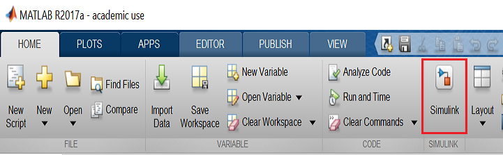
Alternatively, you lot can hit the Simulink push at the top of the MATLAB window as shown hither:

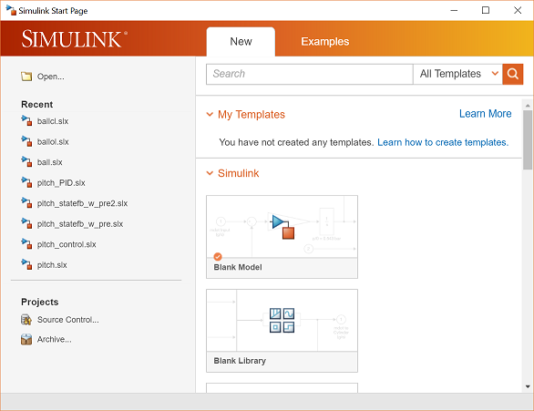
When it starts, Simulink brings up a single window, entitled Simulink Commencement Folio which can be seen here.

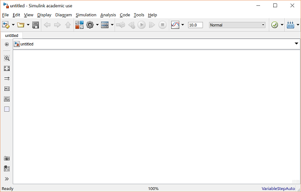
One time you click on Bare Model, a new window will announced as shown below.

Model Files

In Simulink, a model is a collection of blocks which, in general, represents a arrangement. In improver to creating a model from scratch, previously saved model files can exist loaded either from the File carte du jour or from the MATLAB command prompt. As an example, download the following model file by right-clicking on the following link and saving the file in the directory you are running MATLAB from.

unproblematic.slx

Open up this file in Simulink by entering the following command in the MATLAB command window. (Alternatively, you lot tin load this file using the Open option in the File menu in Simulink, or by striking Ctrl-O in Simulink).

simple

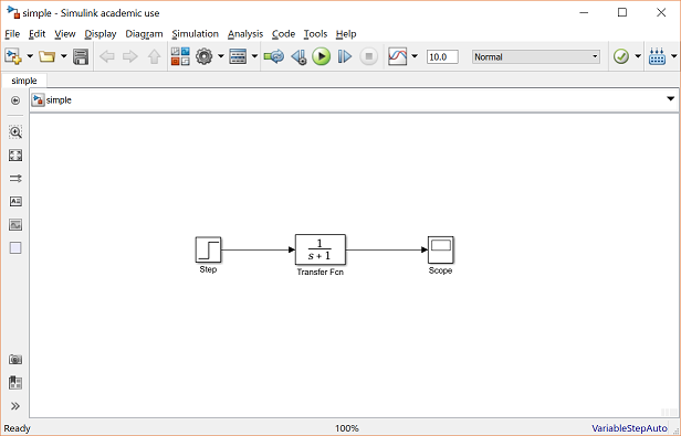
The following model window should appear.

A new model can be created by selecting New from the File menu in any Simulink window (or by hitting Ctrl-Northward).

Bones Elements

There are 2 major classes of items in Simulink: blocks and lines. Blocks are used to generate, modify, combine, output, and display signals. Lines are used to transfer signals from one block to another.

Blocks

There are several general classes of blocks inside the Simulink library:

• Sources: used to generate various signals
• Sinks: used to output or display signals
• Continuous: continuous-time system elements (transfer functions, land-space models, PID controllers, etc.)
• Detached: linear, detached-fourth dimension system elements (discrete transfer functions, discrete country-infinite models, etc.)
• Math Operations: contains many common math operations (gain, sum, product, absolute value, etc.)
• Ports & Subsystems: contains useful blocks to build a system

Blocks take goose egg to several input terminals and zero to several output terminals. Unused input terminals are indicated by a small open triangle. Unused output terminals are indicated by a small triangular signal. The block shown below has an unused input terminal on the left and an unused output terminal on the right.

Lines

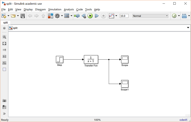
Lines transmit signals in the direction indicated by the arrow. Lines must always transmit signals from the output last of 1 block to the input terminal of another block. On exception to this is a line can tap off of another line, splitting the signal to each of two destination blocks, as shown below (right-click hither and then select Relieve link as ... to download the model file chosen split up.slx).

Lines tin can never inject a signal into another line; lines must be combined through the apply of a block such as a summing junction.

A indicate tin can be either a scalar betoken or a vector point. For Unmarried-Input, Single-Output (SISO) systems, scalar signals are generally used. For Multi-Input, Multi-Output (MIMO) systems, vector signals are often used, consisting of 2 or more scalar signals. The lines used to transmit scalar and vector signals are identical. The blazon of signal carried past a line is determined by the blocks on either stop of the line.

Simple Example

The elementary model consists of three blocks: Step, Transfer Function, and Scope. The Step is a Source block from which a step input indicate originates. This signal is transferred through the line in the direction indicated past the arrow to the Transfer Function Continuous block. The Transfer Part cake modifies its input signal and outputs a new signal on a line to the Scope. The Scope is a Sink cake used to display a signal much like an oscilloscope.

In that location are many more types of blocks available in Simulink, some of which will be discussed after. Right now, we will examine merely the three we have used in the uncomplicated model.

Modifying Blocks

A cake can be modified by double-clicking on information technology. For example, if you lot double-click on the Transfer Role block in the Simple model, y'all will meet the following dialog box.

This dialog box contains fields for the numerator and the denominator of the cake'southward transfer function. By entering a vector containing the coefficients of the desired numerator or denominator polynomial, the desired transfer function tin exist entered. For example, to change the denominator to

(i)

enter the following into the denominator field

[i 2 iv]

and hitting the close push button, the model window will change to the following,

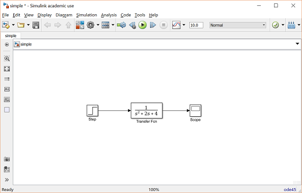
which reflects the change in the denominator of the transfer part.

The Stride block can also be double-clicked, bringing up the following dialog box.

The default parameters in this dialog box generate a stride office occurring at fourth dimension = 1 sec, from an initial level of zero to a level of 1 (in other words, a unit pace at t = 1). Each of these parameters can be inverse. Shut this dialog before continuing.

The most complicated of these three blocks in the Telescopic block. Double-clicking on this brings upwards a blank oscilloscope screen.

When a simulation is performed, the signal which feeds into the telescopic will be displayed in this window. Detailed operation of the scope will not be covered in this tutorial.

Running Simulations

To run a simulation, we volition work with the post-obit model file:

simple2.slx (right-click and then select Save link as ...)

Download and open up this file in Simulink following the previous instructions for this file. You should see the following model window.

Before running a simulation of this arrangement, commencement open up the scope window past double-clicking on the scope cake. Then, to start the simulation, either select Run from the Simulation menu, click the Play push button at the summit of the screen, or hitting Ctrl-T.

The simulation should run very quickly and the scope window volition appear equally shown below.

Annotation that the step response does non begin until t = 1. This can be changed by double-clicking on the step block. Now, nosotros will change the parameters of the system and simulate the arrangement again. Double-click on the Transfer Function block in the model window and change the denominator to:

[one 20 400]

Re-run the simulation (striking Ctrl-T) and yous should meet the following in the telescopic window.

Since the new transfer role has a very fast response, it compressed into a very narrow part of the scope window. This is not really a trouble with the telescopic, merely with the simulation itself. Simulink simulated the organization for a full 10 seconds even though the system had reached steady state presently after one 2d.

To correct this, you need to change the parameters of the simulation itself. In the model window, select Model Configuration Parameters from the Simulation carte du jour. Y'all will see the following dialog box.

In that location are many simulation parameter options; nosotros will but be concerned with the start and stop times, which tell Simulink over what time menstruation to perform the simulation. Alter Start time from 0.0 to 0.8 (since the step doesn't occur until t = 1.0). Modify Stop fourth dimension from 10.0 to 2.0, which should be merely shortly afterward the system settles. Shut the dialog box and rerun the simulation. Now, the scope window should provide a much improve display of the pace response as shown below.

Edifice Systems

In this section, you will learn how to build systems in Simulink using the building blocks in Simulink's Block Libraries. Y'all volition build the post-obit system.

If you would like to download the completed model, right-click here so select Salvage link as ....

Starting time, you will assemble all of the necessary blocks from the block libraries. Then yous will modify the blocks so they stand for to the blocks in the desired model. Finally, you will connect the blocks with lines to form the consummate arrangement. Afterwards this, y'all volition simulate the complete arrangement to verify that it works.

Gathering Blocks

Follow the steps below to collect the necessary blocks:

• Create a new model (New from the File menu or striking Ctrl-N). Y'all volition get a blank model window.
• Click on the Tools tab and so select Library Browser.
• Then click on the Sources listing in the Simulink library browser.

• This will bring up the Sources block library. Sources are used to generate signals.

• Drag the Footstep block from the Sources window into the left side of your model window.

• Click on the Math Operations listing in the main Simulink window.
• From this library, drag a Sum and Proceeds cake into the model window and place them to the correct of the Step cake in that club.
• Click on the Continuous list in the main Simulink window.
• First, from this library, drag a PID Controller block into the model window and identify it to the right of the Gain block.
• From the same library, elevate a Transfer Function block into the model window and place it to the right of the PID Controller block.

• Click on the Sinks listing in the main Simulink window.
• Drag the Scope cake into the right side of the model window.

Modify Blocks

Follow these steps to properly alter the blocks in your model.

• Double-click on the Sum block. Since you will want the second input to be subtracted, enter +- into the list of signs field. Close the dialog box.
• Double-click the Gain cake. Change the gain to ii.5 and close the dialog box.
• Double-click the PID Controller cake and change the Proportional proceeds to 1 and the Integral proceeds to ii. Shut the dialog box.
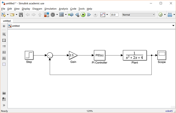
• Double-click the Transfer Role block. Get out the numerator [ane], but modify the denominator to [1 2 iv]. Close the dialog box. The model should announced as:

• Change the proper noun of the PID Controller cake to PI Controller by double-clicking on the word PID Controller.

• Similarly, alter the name of the Transfer Function block to Constitute. At present, all the blocks are entered properly. Your model should appear as:

Connecting Blocks with Lines

Now that the blocks are properly laid out, you will now connect them together. Follow these steps.

• Drag the mouse from the output terminal of the Stride block to the positive input of the Sum input. Another option is to click on the Footstep block and and then Ctrl-Click on the Sum cake to connect the two togther. Yous should see the following.

• The resulting line should have a filled arrowhead. If the arrowhead is open up and red, as shown below, it ways it is non continued to anything.

• Yous tin keep the fractional line you just drew by treating the open arrowhead as an output terminal and drawing but equally before. Alternatively, if you lot want to redraw the line, or if the line connected to the wrong terminal, you should delete the line and redraw it. To delete a line (or any other object), simply click on it to select it, and hit the delete key.
• Draw a line connecting the Sum block output to the Proceeds input. Also draw a line from the Gain to the PI Controller, a line from the PI Controller to the Found, and a line from the Plant to the Scope. You should now have the following.

• The line remaining to exist drawn is the feedback signal connecting the output of the Plant to the negative input of the Sum block. This line is dissimilar in two means. Outset, since this line loops effectually and does not but follow the shortest (right-angled) route and so it needs to be drawn in several stages. Second, at that place is no output terminal to first from, and so the line has to tap off of an existing line.
• Drag a line off the negative portion of the Sum block directly down and release the mouse so the line is incomplete. From the endpoint of this line, click and drag to the line between the Institute and the Scope. The model should now announced equally follows.

• Finally, labels will be placed in the model to place the signals. To place a label anywhere in the model, double-click at the point you want the characterization to be. Start by double-clicking above the line leading from the Step block. You lot volition become a bare text box with an editing cursor as shown beneath.

• Type an r in this box, labeling the reference signal and click outside it to stop editing.
• Label the error (e) indicate, the control (u) signal, and the output (y) signal in the same way. Your final model should appear equally:

To relieve your model, select Relieve Every bit in the File bill of fare and type in any desired model name. The completed model can be downloaded by right-clicking here and so selecting Save link equally ....

Simulation

Now that the model is complete, y'all can simulate the model. Select Run from the Simulation bill of fare to run the simulation. Double-click on the _Scope_block to view its output and you should see the following:

Taking Variables from MATLAB

In some cases, parameters, such every bit gain, may be calculated in MATLAB to be used in a Simulink model. If this is the instance, information technology is not necessary to enter the issue of the MATLAB calculation straight into Simulink. For example, suppose we calculated the gain in MATLAB in the variable M. Emulate this by entering the post-obit command at the MATLAB command prompt.

K = two.5

This variable tin now be used in the Simulink Gain block. In your Simulink model, double-click on the Gain block and enter the following the Gain field.

K

Close this dialog box. Notice now that the Gain block in the Simulink model shows the variable Thousand rather than a number.

Now, y'all can re-run the simulation and view the output on the Scope. The effect should be the same as earlier.

Now, if whatever calculations are done in MATLAB to alter any of the variables used in the Simulink model, the simulation will use the new values the next time information technology is run. To try this, in MATLAB, change the gain, 1000, by entering the following at the command prompt.

K = 5

Commencement the Simulink simulation again and open the Scope window. You will come across the post-obit output which reflects the new, higher gain.

Too variables and signals, even entire systems can be exchanged between MATLAB and Simulink.

All contents licensed under a Creative Commons Attribution-ShareAlike iv.0 International License.

ellardthaps1957.blogspot.com

Source: https://ctms.engin.umich.edu/CTMS/index.php?aux=Basics_Simulink

Share this post